What is a Kalman Filter?

 

Kalman Filter

What is the Attractor Path?

 

What is a Shock Decomposition?

 

The Nixon Shock of 1971 was an attempt to stop inflation by ending convertibility of the US Dollar into Gold. Along with other forms of economic Shock Therapy, is (from the standpoint of Systems Theory) an attempt to pop Economic Bubbles and return the system to a sustainable attractor path. But economies are subject to all sots of shocks and the general question for analysis is how do feedback effects operate in the presence of shocks. The way to study the effects of shocks on a system is called Shock Decomposition And, if you have a computer model, shock decompositions can be studied through computer simulation.

What a shock decomposition will show you depends on (1) what parts of the system are being shocked and (3) the internal dynamics (if any) of the computer model. To focus this discussion, I am going to concentrated on systems and state space models since any system can be put in state space form (see the discussion here).

Take a very simple state space (SS) model:

The SS model state equation (line 1 above) will have p state variables and  m input variables.

World-System (0-2000) The Maddison Database

 The most complete data set on the World-Economy is the one developed by Angus Maddison and published by the OECD (here). I have entered the data into seven spreadsheets for Population, GDP, Urbanization, Real Exports, Exports, Total Hours worked and Employment. The tables are reproduced below.

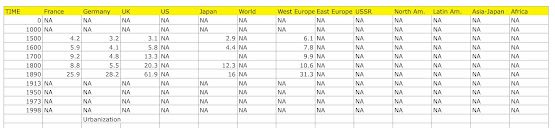
To make continuous series available, I have nonlinearly interpolated missing data using the Spline Smoothing algorithm in the R programming language. Where initial data is missing, I have used the E-M Algorithm to estimate missing values. In some cases for some countries and regions, no data is available.

Boiler Plate

 

State Space Model Estimation

The Measurement Matrix for the state space models was constructed using Principal Components Analysis with standardized data from the World Development Indicators. The statistical analysis was conducted in an extension of the dse package. The package is currently supported by an online portal (here) and can be downloaded, with the R-programming language, for any personal computer here. Code for the state space Dynamic Component models (DCMs) is available on my Google drive (here) and referenced in each post.

Atlanta Fed Economy Now

My approach to forecasting is similar to the EconomyNow model used by the Atlanta Federal Reserve. Since the new Republican Administration is signaling that they would like to eliminate the Federal Reserve, the app might well not be available in the future.

While the app is still available, there have been some interesting developments. In earlier forecasts, the Atlanta Fed was showing GDP growth predictions outside the Blue Chip Consensus. Right now, after unorthodox economic policies from the Trump II Administration, the EconomyNow model is predicting a drastic drop in GDP (the Financial Forecast Center is only predicting a slight drop here).

Climate Change

Another comparison for what I have presented above are the IPCC Emission Scenarios. These scenarios are for the World System. Needless to say, (1) the new Right-Wing Republican administration plans on withdrawing the US from all attempts to study or ameliorate Climate Change and (2) the IPCC does not produce any RW modes for the World System (but seem my forecasts here).

World System

The longest running set of data we have for the World-System is the Maddison Project based on the work of Angus Maddison (more information is available here). Data on production (Q) and population (N) for most countries and regions runs from years 0-2000. More data becomes available as we near the year 2000. 

Available data were entered in a spreadsheet (see Population above, double click to enlarge). Missing data were interpolated with nonlinear spline smoothing using the R programming Language.

In cases where initial values were not available (see GDP above), the E-M Algorithm was used to estimate initial conditions.

From the graph of GDP above (W_Q) for the World System, it can be seen that economic growth from the year 0-1500 was basically flat. The period of British Capitalism (after 1500) had a small plateau of growth. Takeoff does not happen until the Nineteenth Century.

From a system's perspective, the only model that can be tested for the entire period is Kenneth Boulding's Malthusian Systems Model [Q,N] = f[Q,N].

When developed as a State Space model (measurement matrix above) there are two components: W1=Growth and W2=(Q-N), the Malthusian Controller. When more data is available, the Malthusian Controller can be generalized to other SocioEconomic theories.

What the Malthusian Controller shows (plotted as Q-N above) is that a long-developing Malthusian Crisis (Q<N) started in the Late Middle Ages and accelerated through the period of British Capitalism (Dark Satanic Mills) and was reversed spectacularly during the Nineteenth Century.  Takeoff in response to a deepening Malthusian Crisis would not be an unreasonable way to view Modern Economic Growth.

Error Correcting Controllers (ECC)

In another post (here), I presented Leibenstein's Malthusian Error Correcting Controller (ECC). It can be generalized to the dominant ECCs in most theoretical economic models (above). These controllers can be further generalized. For example, (X-U) and (L-U) can be generalized to (N-U), a more general Urbanization Controller which describes market expansion for economic growth. In countries and periods with limited data, (N-U) might subsume all these processes. ECCs describe important feedback processes in SocioTechnical System that are typically not recognized as such in academic literature.

Kaya Identity

The basic theoretical model underlying all the World-System models I create is the Kaya Identity. There are a number of advantages to starting theoretical development with the Kaya Identity: (1) An "identity" is true by definition Adding other variables to the model ensure that theory construction is on a solid footing. (2) The Kaya Identity is used as the basis for the IPCC Emission Scenarios.

World Development Indicators (WDI)

After WWII, extensive data sets on all countries in the World-System became available from the World Bank (here). The indicators above where chose to construct the state space for each WDI-based model. Addition indicators can be added for specific forecasts and analyses.

Dynamic Component Models (DCMs)

 

The Dynamic Components Model (DCM) is a form of State Space Model where the approximate state variables are first computed using Principal Components Analysis (PCA). The difference between a standard State Space Model and the DCM are (1) how the Measurement Matrix (see graphic above) is computed (with PCA) and (2) how the state variables are analyzed directly. The advantage of the DCM is that it separates the growth and control state variables so that growth and control can be analyzed independently (the PCs are statistically independent). In the Cannonical DCM, there are only three state variables (one for growth and one for control) that explain at least 80% of the variation in the Output Variables. The control components are typical made up of Error Correcting Controllers (ECCs). In SocioEconomic systems the ECCs are typically associated with a theoretical tradition. For example, the Malthusian Controller is presented here and generalized here. ECCs are key elements of Cybernetics and the dominant growth component is a key element of Systems Theory and Economic Growth Theory.

The DCM is implemented in the public domain R Programming language as an extension to the dse (Dynamic System Estimation) package. The dse package can be downloaded on all Computer platforms and can be run on line with a web browser (here). The DCM extensions with documentation are available here.

In the dse package, a state space model can be created using the SS command in R:

The State Space model has two forms: non-innovations and innovations:

The matrices are (double click to enlarge):

An example of the USL20 model can be found here. Other examples of the models with written analysis can be found on my blog at Blogger.com (here). For more information on Dynamic Component Models see Pasdirtz, 2007.

Properties of State Space Models

Stability

Mechanization

Controllability

Reachability

Stability

McMillan Degree