Sunday, October 14, 2012

HLMs: The ML Estimator

In a prior post (here) I wrote out two models for the Dyestuff data set. The first model was a simple regression model and the second model was a hierarchical, random-coefficients model. I first estimated the simple regression model which does not contain random components. In this post, I will estimate the standard Maximum Likelihood (ML) model used to fit random components and hierarchal models.

The lme4 package has been developed by Doug Bates at the University of Wisconsin and is considered state-of-the-art for ML estimation of mixed models, that is, models with both fixed and random effects, such as hierarchical models. Package documentation is available here, draft chapters of a book on lme4 are available here and an excellent presentation on lme4 given at the UseR!2008 Conference is available here.

In Chapter 1 of the lme4() book, Doug Bates is careful to clear up the terminological problems that have plagued the statistics literature:
  • Mixed-Effects Models describe a relationship between a response (dependent) variable and the covariates (independent variables). However, a mixed-effects model contains both fixed- and random-effects as independent variables. Furthermore, one of the covariates must be a categorical variable representing experimental or observational units (the units of analysis).
  • Fixed-effect Parameters are parameters associated with a covariate that is fixed and reproducible, meaning under experimental control.
  • Random Effects are levels of a covariate that are a random sample from all possible levels of the covariate that might have been included in the model.
In the Dyestuff data set, the experimental unit is the batch of intermediate product used in creating a dye. Part of the confusion in terminology is that "fixed" and "random" are more a property of the levels rather than the effects. And, although there are fixed effect parameters, the random effects are not parameters. Confused?


To me, the confusion is cleared up by returning to the model and considering the terminology an attribute of the model rather than the data. In the model above, lambda 00 is the fixed effect and mu 0j is the random effect which is simply the error term on the first equation. Since both mu 0j and epsilon ij are error terms, they are not parameters in the model. On the other hand, sigma u0 and sigma e are parameters. Still confused?

What I will argue repeatedly in remaining posts is that the way you determine what is or is not a parameter is through Monte Carlo simulation. For a given model, terms that must be fixed before you can run the simulation are parameters. Other terms in the model are random variables, that is, simulation variables that we will have to generate from some density function. What I insist to my students is that you cannot use input data to run the Monte Carlo simulation.  In order for the simulation to work without input data, you must be clear about (and often surprised by) the actual random variables in your model.

Before I present the ML model in the notation Doug Bates is using, let's return to the expanded Dyestuff hierarchical model introduced earlier.


In the HLM-form of the Dyestuff model, the matrix Z codes different manufacturers, the second level variable.  When we solve the model in the third equation above we see that an interaction term between ZX has been added to the model.


Laird and Ware (1982) (you can find the article here, but let me know if this link is broken) develop another popular form of the model in the equations above. In Stage 2, as they call the second level, the b matrix of unknown individual effects is distributed normally with covariance matrix D. The population parameters, the alpha matrix, are treated as fixed effects. In Stage 1, each individual unit i follows the second equation above: e is distributed N(0,R) where R is the covariance matrix. At this stage, the alpha and the beta matrices are considered fixed.

In the marginal distribution, (|  b), the y are also independent normals with covariance matrix R + Z D Z' where R, under conditions of conditional independence, can be simplified to an identity matrix with a single standard error, sigma.

The Laird and Ware (1982) article is worth detailed study. They present not only the ML model but also the Bayesian approach that leads to the restricted maximum likelihood (REML) estimator. And, they explain clearly how the EM (expectation-maximization) algorithm can be used to solve the model. The EM algorithm treats the individual characteristics of random effects models as missing data where the expected value replaces each missing data element after which the effects are re-estimated until the likelihood is maximized. I will talk about the EM algorithm in a future post because it is the best approach to deal generally with missing data.
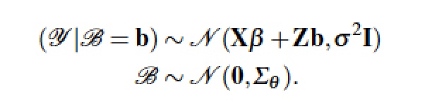
Finally, we get to Doug Bates' notation, which should be clearer now that we have presented the Laird and Ware model. What is important to note is that Doug assumes conditional independence.

Although I love matrix algebra, for HLMs I prefer to write out models explicitly in non-matrix terms as was done in the first set of equations above. In the lme4 package, my students have found the notation for specifying the random components of the model in the Z matrix to be somewhat confusing. Returning to the single-equation HLM form of their models has help to clear up the confusion.

> fm1 <- lmer(Yield ~ 1 + (1|Batch),Dyestuff)
> summary(fm1)
Linear mixed model fit by REML 
Formula: Yield ~ 1 + (1 | Batch) 
   Data: Dyestuff 
   AIC   BIC logLik deviance REMLdev
 325.7 329.9 -159.8    327.4   319.7
Random effects:
 Groups   Name        Variance Std.Dev.
 Batch    (Intercept) 1764.0   42.001  
 Residual             2451.3   49.510  
Number of obs: 30, groups: Batch, 6

Fixed effects:
            Estimate Std. Error t value
(Intercept)  1527.50      19.38   78.81

The Dyestuff model is specified in the lme4() procedure with the equation Yield ~ 1 + (1|Batch). The random effects in the parentheses are read "the effect of Batch given the grand mean". It may seem strange to find the grand mean (represented by the 1) specified twice in a model. Going back to the single equation HLM form, notice that there are two constants, lambda 00 and the first element of the beta 0 j matrix, thus the two grand means.

Moving beyond the notation to the estimated values, we have two standard errors (42.001, and 49.510) and one fixed effect parameters, 1527.50 with standard error 19.38. The "Random effects: Residual" is the same residual standard deviation, 49.510, as from the OLS ANOVA. That's a little disconcerting because, they way the initial model was written, it would seem that the residual standard deviation should be smaller when we have taken the random error components out of the OLS estimate.

> coef(m1)[1] + mean(coef(m1)[2:6])
(Intercept) 
       1532 

The fixed effect mean is very similar to the average of the OLS coefficients. So, all this heavy machinery was developed to generate the one number, 42.001. Here's my question: "Is this the right number?" I will argue in the next post that the only way to answer this question is through Monte Carlo simulation.

NOTE: Another way to think about random and fixed effects is to think about the problem of prediction. If we want to predict the Yield we might get from a future batch of dyestuff from some manufacturer, all we have to work with are the fixed part of the models. The random components are unique to the sample and will not be reproduced in future samples. We can use the standard deviations and the assumed density functions (usually normal) to compute confidence intervals, but the predicted mean values can only be a function of the fixed effects.

Monday, September 24, 2012

The Dyestuff Model

In a prior post (here), I introduced the Dyestuff data set. At first, one might be tempted to run an analysis of variance (ANOVA) on this data since the stated intention is to analyze variation from batch to batch. The ANOVA model is equivalent to the standard regression model.


Here, all the terms represent matrices: Y is an (n x 1) matrix of dependent variables, Yield in this case.  X is an (n x m) design matrix (to be explained in the NOTE below) coding the Batch. The beta matrix is a (m x 1) matrix of unknown coefficients. And, the e matrix is an (n x 1) matrix of unknown errors (departures from perfect fit) distributed normally with mean zero and a single variance, sigma. If your matrix algebra is weak, R provides a great environment for learning linear algebra (see for example here).

The regression model is completely equivalent to ANOVA. You can convince yourself of this by running the two analyses in R.


> m1 <- lm(Yield ~ Batch,Dyestuff,x=TRUE)
> summary(m1)

Call:
lm(formula = Yield ~ Batch, data = Dyestuff, x = TRUE)

Residuals:
   Min     1Q Median     3Q    Max 
-85.00 -33.00   3.00  31.75  97.00 

Coefficients:
            Estimate Std. Error t value Pr(>|t|)    
(Intercept)  1505.00      22.14  67.972  < 2e-16 ***
BatchB         23.00      31.31   0.735  0.46975    
BatchC         59.00      31.31   1.884  0.07171 .  
BatchD         -7.00      31.31  -0.224  0.82500    
BatchE         95.00      31.31   3.034  0.00572 ** 
BatchF        -35.00      31.31  -1.118  0.27474    
---
Signif. codes:  0 ‘***’ 0.001 ‘**’ 0.01 ‘*’ 0.05 ‘.’ 0.1 ‘ ’ 1 

Residual standard error: 49.51 on 24 degrees of freedom
Multiple R-squared: 0.4893, Adjusted R-squared: 0.3829 
F-statistic: 4.598 on 5 and 24 DF,  p-value: 0.004398 

> anova(m1)
Analysis of Variance Table

Response: Yield
          Df Sum Sq Mean Sq F value   Pr(>F)   
Batch      5  56358 11271.5  4.5983 0.004398 **
Residuals 24  58830  2451.2                    
---
Signif. codes:  0 ‘***’ 0.001 ‘**’ 0.01 ‘*’ 0.05 ‘.’ 0.1 ‘ ’ 1 


In R, the anova(m1) command produces the same results as summary(m1), only the results are presented as the standard ANOVA table.

The naive regression result finds that the means of Batches C and E are significantly different from the other batches. What the result says for the initial question is that most batches are +/- 31.31 units from the average yield of 1505. However, some batches can be significantly outside this range. But, is this an analysis of means or analysis of variances?  The history and development of terminology (analysis-of-variance, analysis of means, random error terms, random components, random effects, etc.) makes interesting reading that I will explore in a future post. To maintain sanity, it's important to keep focused on the model rather than the terminology.

If we write out another model that might have generated this data, it becomes easier to clarify terminology and understand why ANOVA (analysis of means) might not be the right approach to analyze the  variation from batch to batch.


Since we have no control over the sampling of batches, we expect that the Yield coefficient will have a random source of variation in addition to the true population yield (see the first equation above). Under normal experimental conditions we might try to randomize away this source of variation by sampling batches for a wide range of suppliers. But, since we are actually not using random assignment, we have a unique source of variation associated with the yield of each batch. As can be seen from the first equation above, this is where the term random coefficients comes from.  Where we have random sampling, the effect of Batch on Yield would be a fixed effect, that is, fixed under sampling. In this model, the fixed effect is lambda_00 rather than the usual beta.

The equation that determines Yield (the second and third equations above) thus has a random coefficient. If we substitute Equation 1 into Equation 2, we get Equation 4. Notice that we now have a larger error term, one error associated with Batch and another associated with the model. The purpose of hierarchical modeling is to account for the source of error associated with how the Batches are generated. The "analysis of variance" here involves the two sigma parameters, sigma_u0 (the standard error of the yield coefficient) and sigma_e (the standard error of the regression).


What you might be asking yourself right now is "If this is a HLM, where's the hierarchy?" Let's assume that we were receiving batches from more than one manufacturer. Then, we would have batches nested within suppliers, but still no random sampling. To account for the effect of supplier, we need another second-level variable (second level in the hierarchy), Z, that is an indicator variable identifying the manufacturer.


The organizational chart above makes the hierarchy explicit. If we take the Z out of the model, however, we are still left with a random coefficients model. Since most human activity is embedded within some social hierarchy, it is hard to find a unit of analysis that is not hierarchical: (1) students within class rooms, classrooms within schools, schools within school systems, etc., (2) countries nested within regions, (3) etc. When these implicit hierarchies are not modeled, a researcher can only hope that the second-level random effects are small.

Returning to terminology for a moment, if we were just interested in the analysis of means, then standard ANOVA models (sometimes called Type I ANOVA) gives us a fairly good analysis of differences in Yield. We might have more error associated with the non-random Batches in the error term, but we still have significant results (some Batches have significantly different means in spite of the unanalyzed  sources of Batch variance). However, if we are interested in true analysis of variance (sometimes called Type II ANOVA) and if we expect that there is some unique source of variation associated with Batches that we want to analyze, we need a technique that will produce estimates of both sigma_u0 (the standard error of the yield coefficient) and sigma_e (the standard error of the regression).

There are multiple techniques that will perform a Type II ANOVA or random coefficients analysis. In the next post I'll discuss the most popular approach, Maximum Likelihood Estimation (MLE).

NOTE: The equivalence of ANOVA and regression becomes a little clearer by looking at the  design matrix for the Dyestuff model. Most students are familiar with the standard regression model where the independent variable, X, is an (n x 1) matrix containing values for a continuous variable. This is how the difference between ANOVA and regression is typically explained in introductory text books. However, if the X matrix contains dummy [0,1] variables coding each Batch, the regression model is equivalent to ANOVA. Here is the design matrix, as the ANOVA X matrix is often called, for the Dyestuff model:


> m1$x
   (Intercept) BatchB BatchC BatchD BatchE BatchF
1            1      0      0      0      0      0
2            1      0      0      0      0      0
3            1      0      0      0      0      0
4            1      0      0      0      0      0
5            1      0      0      0      0      0
6            1      1      0      0      0      0
7            1      1      0      0      0      0
8            1      1      0      0      0      0
9            1      1      0      0      0      0
10           1      1      0      0      0      0
11           1      0      1      0      0      0
12           1      0      1      0      0      0
13           1      0      1      0      0      0
14           1      0      1      0      0      0
15           1      0      1      0      0      0
16           1      0      0      1      0      0
17           1      0      0      1      0      0
18           1      0      0      1      0      0
19           1      0      0      1      0      0
20           1      0      0      1      0      0
21           1      0      0      0      1      0
22           1      0      0      0      1      0
23           1      0      0      0      1      0
24           1      0      0      0      1      0
25           1      0      0      0      1      0
26           1      0      0      0      0      1
27           1      0      0      0      0      1
28           1      0      0      0      0      1
29           1      0      0      0      0      1
30           1      0      0      0      0      1
attr(,"assign")
[1] 0 1 1 1 1 1
attr(,"contrasts")
attr(,"contrasts")$Batch
[1] "contr.treatment"


Notice that there is no BatchA, since it plays the role of the reference class to which other batches are compared. That is, the coefficients attached to BatchB through BatchF are expressed as deviations from the grand mean (this construction is necessary because there are only 6 parameters and 6 degrees of freedom, so one class has to become the grand mean).