HLMs: The ML Estimator

In a prior post (here) I wrote out two models for the Dyestuff data set. The first model was a simple regression model and the second model was a hierarchical, random-coefficients model. I first estimated the simple regression model which does not contain random components. In this post, I will estimate the standard Maximum Likelihood (ML) model used to fit random components and hierarchal models.

The lme4 package has been developed by Doug Bates at the University of Wisconsin and is considered state-of-the-art for ML estimation of mixed models, that is, models with both fixed and random effects, such as hierarchical models. Package documentation is available here, draft chapters of a book on lme4 are available here and an excellent presentation on lme4 given at the UseR!2008 Conference is available here.

In Chapter 1 of the lme4() book, Doug Bates is careful to clear up the terminological problems that have plagued the statistics literature:

• Mixed-Effects Models describe a relationship between a response (dependent) variable and the covariates (independent variables). However, a mixed-effects model contains both fixed- and random-effects as independent variables. Furthermore, one of the covariates must be a categorical variable representing experimental or observational units (the units of analysis).
• Fixed-effect Parameters are parameters associated with a covariate that is fixed and reproducible, meaning under experimental control.
• Random Effects are levels of a covariate that are a random sample from all possible levels of the covariate that might have been included in the model.

In the Dyestuff data set, the experimental unit is the batch of intermediate product used in creating a dye. Part of the confusion in terminology is that "fixed" and "random" are more a property of the levels rather than the effects. And, although there are fixed effect parameters, the random effects are not parameters. Confused?

To me, the confusion is cleared up by returning to the model and considering the terminology an attribute of the model rather than the data. In the model above, lambda 00 is the fixed effect and mu 0j is the random effect which is simply the error term on the first equation. Since both mu 0j and epsilon ij are error terms, they are not parameters in the model. On the other hand, sigma u0 and sigma e are parameters. Still confused?

What I will argue repeatedly in remaining posts is that the way you determine what is or is not a parameter is through Monte Carlo simulation. For a given model, terms that must be fixed before you can run the simulation are parameters. Other terms in the model are random variables, that is, simulation variables that we will have to generate from some density function. What I insist to my students is that you cannot use input data to run the Monte Carlo simulation.  In order for the simulation to work without input data, you must be clear about (and often surprised by) the actual random variables in your model.

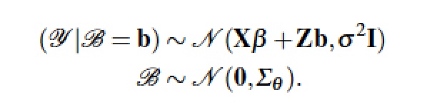
Before I present the ML model in the notation Doug Bates is using, let's return to the expanded Dyestuff hierarchical model introduced earlier.

In the HLM-form of the Dyestuff model, the matrix Z codes different manufacturers, the second level variable.  When we solve the model in the third equation above we see that an interaction term between ZX has been added to the model.

Laird and Ware (1982) (you can find the article here, but let me know if this link is broken) develop another popular form of the model in the equations above. In Stage 2, as they call the second level, the b matrix of unknown individual effects is distributed normally with covariance matrix D. The population parameters, the alpha matrix, are treated as fixed effects. In Stage 1, each individual unit i follows the second equation above: e is distributed N(0,R) where R is the covariance matrix. At this stage, the alpha and the beta matrices are considered fixed.

In the marginal distribution, (y |  b), the y are also independent normals with covariance matrix R + Z D Z' where R, under conditions of conditional independence, can be simplified to an identity matrix with a single standard error, sigma.

The Laird and Ware (1982) article is worth detailed study. They present not only the ML model but also the Bayesian approach that leads to the restricted maximum likelihood (REML) estimator. And, they explain clearly how the EM (expectation-maximization) algorithm can be used to solve the model. The EM algorithm treats the individual characteristics of random effects models as missing data where the expected value replaces each missing data element after which the effects are re-estimated until the likelihood is maximized. I will talk about the EM algorithm in a future post because it is the best approach to deal generally with missing data.

Finally, we get to Doug Bates' notation, which should be clearer now that we have presented the Laird and Ware model. What is important to note is that Doug assumes conditional independence.

Although I love matrix algebra, for HLMs I prefer to write out models explicitly in non-matrix terms as was done in the first set of equations above. In the lme4 package, my students have found the notation for specifying the random components of the model in the Z matrix to be somewhat confusing. Returning to the single-equation HLM form of their models has help to clear up the confusion.

> fm1 <- lmer(Yield ~ 1 + (1|Batch),Dyestuff)

> summary(fm1)

Linear mixed model fit by REML 

Formula: Yield ~ 1 + (1 | Batch) 

   Data: Dyestuff 

   AIC   BIC logLik deviance REMLdev

 325.7 329.9 -159.8    327.4   319.7

Random effects:

 Groups   Name        Variance Std.Dev.

 Batch    (Intercept) 1764.0   42.001  

 Residual             2451.3   49.510  

Number of obs: 30, groups: Batch, 6

Fixed effects:

            Estimate Std. Error t value

(Intercept)  1527.50      19.38   78.81

The Dyestuff model is specified in the lme4() procedure with the equation Yield ~ 1 + (1|Batch). The random effects in the parentheses are read "the effect of Batch given the grand mean". It may seem strange to find the grand mean (represented by the 1) specified twice in a model. Going back to the single equation HLM form, notice that there are two constants, lambda 00 and the first element of the beta 0 j matrix, thus the two grand means.

Moving beyond the notation to the estimated values, we have two standard errors (42.001, and 49.510) and one fixed effect parameters, 1527.50 with standard error 19.38. The "Random effects: Residual" is the same residual standard deviation, 49.510, as from the OLS ANOVA. That's a little disconcerting because, they way the initial model was written, it would seem that the residual standard deviation should be smaller when we have taken the random error components out of the OLS estimate.

> coef(m1)[1] + mean(coef(m1)[2:6])

(Intercept) 

       1532 

The fixed effect mean is very similar to the average of the OLS coefficients. So, all this heavy machinery was developed to generate the one number, 42.001. Here's my question: "Is this the right number?" I will argue in the next post that the only way to answer this question is through Monte Carlo simulation.

NOTE: Another way to think about random and fixed effects is to think about the problem of prediction. If we want to predict the Yield we might get from a future batch of dyestuff from some manufacturer, all we have to work with are the fixed part of the models. The random components are unique to the sample and will not be reproduced in future samples. We can use the standard deviations and the assumed density functions (usually normal) to compute confidence intervals, but the predicted mean values can only be a function of the fixed effects.