Two earlier posts (here and here) described a simple hierarchical linear model (HLM) for Black Friday Retail Sales using data from an article in the Washington Post (here). The pedagogical purpose of the HLM exercise was to display one answer to Simpson's Paradox. It wasn't meant to be a general recommendation for the analysis of retail sales.
The analysis of aggregate retail sales is essentially a time series problem in that we are analyzing sales over time for, ideally, multiple years. HLMs can be written to handle time series problems, a topic that I will return to in a later post. The analysis of aggregate US retail sales, however, can be analyzed with a straight-forward state space time series model. If you are interested in the pure time series approach, I have done that in another post (here).
The insight from the time series analysis is that US Retail Sales are being driven by the World economy which makes sense in a world of globalized retail trade. The idea that Black Friday Sales might be a good predictor of aggregate retail sales is, based on purely theoretical considerations, not a very appealing hypothesis.
Friday, December 28, 2012
Friday, December 7, 2012
How to Write Hierarchical Model Equations
In the last few posts (here and here) I've written out systems of equations for hierarchical models. So far, I've written out equations for the Dyestuff and the Black Friday Sales models. Hopefully, it's easy to follow the equations once they are written out. Starting from scratch and writing your own equations might be another matter. In this post I will work through some examples that should give some idea about how to start.
First, I will review the examples I have already used and in future posts introduce a few more. When I develop equations, there is an interaction between how I write the equations and how I know I will have to write simulation code to generate data for the model. Until I actually show you how to write that R code in a future post, I'm going to use pseudo-code, that is, an English language (rather than machine readable) description of the algorithm necessary to generate the data. If you have not written pseudo-code before, Wikipedia provides a nice description with a number of examples of "mathematical style pseudo-code" (here).
For the Dyestuff example (here and here) we were "provided" six "samples" representing different "batches of works manufacturer." The subtle point here is that we are not told that the batches were randomly sampled from the universe of all batches we might receive at the laboratory (probably an unrealistic and impossible sampling plan). So, we have to deal with each batch as a unit without population characteristics. So, I can start with the following pseudo-code:
For (Every Batch in the Sample)
For (Every Observation in the Batch)
Generate a Yield coefficient from a batch distribution.
Generate a Yield from a sample distribution.
End (Batch)
End (Sample)
If we had random sampling, I would have been able to simply generate a Yield from a sample Yield Coefficient and a sample Yield distribution (the normal regression model). What seems difficult for students is that many introductory regression texts are a little unclear about how the data were generated. On careful examination, examples turn out to not have been randomly sampled from some large population. Hierarchical models, and the attempt to simulate the underlying data generation process, sensitize us to the need for a more complicated representation. So, instead of the single regression equation we get a system of equations:

where lambda_00 is the yield parameter, mu_0j is the batch error term, beta_0j is the "random" yield coefficient, X is the batch (coded as a dummy variable matrix displayed here), epsilon_ij is the sample error and Y_ij is the observed yield. With random sampling, beta_0j would be "fixed under sampling" at the sample level. Without random sampling, it is a "random coefficient". Here, the batch and the sample distributions are both assumed to be normal with mean 0 and standard errors sigma_u0 and sigma_e, respectively. I'll write the actual R code to simulate this data set in the next post.
The second model I introduced was the Black Friday Sales model (here). I assumed that we have yearly weekly sales data and Black Friday week sales generated at the store level. I also assume that we have retail stores of different sizes. In the real world, not only do stores of different sizes have different yearly sales totals but they probably have somewhat different success with Black Friday Sales events (I always seem to see crazed shoppers crushing into a Walmart store at the stroke of midnight, for example here, rather than pushing their way into a small boutique store). For the time being, I'll assume that all stores have the same basic response to Black Friday Sales just different levels of sales. In pseudo-code:
For (Each Replication)
For (Each Size Store)
For (Each Store)
Generate a random intercept term for store
Generate Black Friday Sales from some distribution
Generate Yearly Sales using sample distribution
End (Store)
End (Store Size)
End (Replication)
and in equations

where the terms have meanings that are similar to the Dyestuff example.
I showed the actual R code for generating a Black Friday Sales data set in the last post (here). The two important equations to notice within the outer loops are
b0 <- b[1] - store + rnorm(1,sd=s[1])
yr.sales <- b0 + b[2]*bf.sales + rnorm(1,sd=s[2])
The first gets the intercept term using a normal random number generator and the second forecasts the actual yearly sales using a second normal random number generator. The parameters to the function rnorm(1,sd=s[1],mean=0) tell the random number generator to generate one number with mean zero (the default) and standard deviation given s[1]. For more information on the random number generators in R type
> help(rnorm)
after the R prompt (>). In a later post I will describe how to generate random numbers from any arbitrary or empirically generated distribution using the hlmmc package. For now, standard random numbers will be just fine.
In the next post I'll describe in more detail how to generate the Dyestuff data.
First, I will review the examples I have already used and in future posts introduce a few more. When I develop equations, there is an interaction between how I write the equations and how I know I will have to write simulation code to generate data for the model. Until I actually show you how to write that R code in a future post, I'm going to use pseudo-code, that is, an English language (rather than machine readable) description of the algorithm necessary to generate the data. If you have not written pseudo-code before, Wikipedia provides a nice description with a number of examples of "mathematical style pseudo-code" (here).
For the Dyestuff example (here and here) we were "provided" six "samples" representing different "batches of works manufacturer." The subtle point here is that we are not told that the batches were randomly sampled from the universe of all batches we might receive at the laboratory (probably an unrealistic and impossible sampling plan). So, we have to deal with each batch as a unit without population characteristics. So, I can start with the following pseudo-code:
For (Every Batch in the Sample)
For (Every Observation in the Batch)
Generate a Yield coefficient from a batch distribution.
Generate a Yield from a sample distribution.
End (Batch)
End (Sample)
If we had random sampling, I would have been able to simply generate a Yield from a sample Yield Coefficient and a sample Yield distribution (the normal regression model). What seems difficult for students is that many introductory regression texts are a little unclear about how the data were generated. On careful examination, examples turn out to not have been randomly sampled from some large population. Hierarchical models, and the attempt to simulate the underlying data generation process, sensitize us to the need for a more complicated representation. So, instead of the single regression equation we get a system of equations:

The second model I introduced was the Black Friday Sales model (here). I assumed that we have yearly weekly sales data and Black Friday week sales generated at the store level. I also assume that we have retail stores of different sizes. In the real world, not only do stores of different sizes have different yearly sales totals but they probably have somewhat different success with Black Friday Sales events (I always seem to see crazed shoppers crushing into a Walmart store at the stroke of midnight, for example here, rather than pushing their way into a small boutique store). For the time being, I'll assume that all stores have the same basic response to Black Friday Sales just different levels of sales. In pseudo-code:
For (Each Replication)
For (Each Size Store)
For (Each Store)
Generate a random intercept term for store
Generate Black Friday Sales from some distribution
Generate Yearly Sales using sample distribution
End (Store)
End (Store Size)
End (Replication)
and in equations
where the terms have meanings that are similar to the Dyestuff example.
I showed the actual R code for generating a Black Friday Sales data set in the last post (here). The two important equations to notice within the outer loops are
b0 <- b[1] - store + rnorm(1,sd=s[1])
yr.sales <- b0 + b[2]*bf.sales + rnorm(1,sd=s[2])
The first gets the intercept term using a normal random number generator and the second forecasts the actual yearly sales using a second normal random number generator. The parameters to the function rnorm(1,sd=s[1],mean=0) tell the random number generator to generate one number with mean zero (the default) and standard deviation given s[1]. For more information on the random number generators in R type
> help(rnorm)
after the R prompt (>). In a later post I will describe how to generate random numbers from any arbitrary or empirically generated distribution using the hlmmc package. For now, standard random numbers will be just fine.
In the next post I'll describe in more detail how to generate the Dyestuff data.
Thursday, December 6, 2012
Generating Hierarchical Black Friday Data
Following up on my last post (here), I'll show how to generate hierarchical Black Friday data. The reason for starting from scratch and trying to simulate your own data is that it helps clarify the data generating process. In the real world, we really don't know how data are generated. In a simulated world, we know exactly how the data are generated. We can then explore different estimation algorithms to see which one gives the best answer.
My guess is that Paul Dales of Capital Economics chose regression analysis because he was testing, in a straight-forward way, whether Black Friday store sales could be used to predict yearly store sales. The problem is that, even though this can be stated as a regression equation, it does not describe how the process actually works. Black Friday sales are generated at the store level as are all the other weekly sales for the year. I'll show how that data-generating model should be written below.
Since this posting is meant to show you how to generate your own Black Friday data set, load the hlmmc libraries and procedures as usual in the R console window (using the hlmmc package is described here and the R programming language, a free multi-platform public-domain program, is available here):
> setwd(W <- "absolute path to your working directory")
> source(file="LibraryLoad.R")
> source(file="HLMprocedures.R")


To make things simple to start (I'll explain how to make it more complicated in a future post), assume that the red store lines are all parallel. In terms of a regression equation, the only difference between these lines then is in the constant term.
The first equation above models that term. (Store) is an indicator variable which is zero for the largest store (imagine it's Target). Lambda_00 plus some normally distributed error term, mu_0j, determines the intercept value for that store. To create data that looked like Paul Dales', I chose a value of 1.3 for lambda_00. The smallest store (imagine a small, hip, boutique shop) was coded 3 since it was the fourth type of store by size and would have an intercept that was 3 less than Target plus some error term. Stores of other sizes would fall in between. The regression lines would all be the same with a value chosen at Beta_1j = 0.6 in the second equation.
I chose the Black Friday Sales value (the X in the second equation) by generating a uniform random number between -2 and 0 (the approximate values for the biggest store, say Target) and then shifted the value upward based on the store number (the details of this are presented in the code below). The modeling assumes that, as part of our sampling plan, we deliberately chose stores of different sizes (again, I have no idea how the original stores were sampled by Mr. Dales but the simulation exercise is designed to make me think about the issue).
The third equation above is the naive regression equation used in Paul Dales' analysis. By substituting in our more realistic data generating model in the fourth equation we see that we actually have two error terms, mu_0j and epsilon_ij. This result should sensitize us to the possibility that we might not find significant results in a naive regression model if the data were really generated hierarchically with error both at the store- and aggregate-levels .
Hopefully, the data generating model is now clear and we can start creating some simulated data. In the R console window you can type the following (after the prompt >):
> data <- BlackFriday(5,b=c(1.3,.6),s=c(.1,.1))
> print(data)
rep store yr.sales bf.sales
1 1 0 0.60498656 -1.28033788
2 1 1 0.42855766 0.55819436
3 1 2 0.44069794 1.75098032
4 1 3 -1.13941544 1.15851739
5 2 0 0.67690293 -0.76659779
6 2 1 -0.02461608 -0.70585148
7 2 2 -0.29758061 0.94070016
8 2 3 -0.81785998 1.30860288
9 3 0 0.73137890 -0.76108426
10 3 1 0.10962475 0.03706152
11 3 2 -0.25702733 0.78483895
12 3 3 -0.26299819 2.27981412
13 4 0 0.18242785 -1.83775363
14 4 1 0.58905336 0.42490799
15 4 2 -0.10427473 1.13952646
16 4 3 -0.59097226 2.01763782
17 5 0 1.00266302 -0.51554774
18 5 1 0.29517583 0.17561673
19 5 2 0.07723300 1.06761291
20 5 3 -0.20515208 2.67945502
> naive.model <- lm(yr.sales ~ bf.sales,data)
> lmplot(naive.model,data,xlab="Black Friday Store Sales",ylab="Yearly Store Sales")
> htsplot(yr.sales ~ bf.sales | store,data,xlab="Black Friday Store Sales",ylab="Yearly Store Sales")
>


The next command computes and plots (above) a separate regression line for each store. These lines all have a positive slope, each one somewhat different due to random error. Thus, at the store level, Black Friday sales are a good predictor of yearly sales while at the aggregate level, the relationship is negative or even non-existant as Mr. Dales reports. Which answer is right?
The answer to that question depends on your point of view. From the standpoint of the US retail sector, maybe Black Friday is 'a bunch of meaningless hype'. From each store's perspective, however, it is a very important sales day and explains why a lot of effort is put into the promotion. The reason the aggregate regression line is negative is simply that there are stores of different sizes in the aggregate sample. Total yearly sales are smaller in smaller stores.
Remember, I have no idea how Paul Dales generated his data, what the sampling plan was or where the data came from (stores or a government agency). It could just as easily be the case that the individual Black Friday store sales are negatively related to yearly sales, contradicting Economics 101. Before we can make this spectacular assertion, however, the data has to be analyzed at the store level with a hierarchical model.
I'll describe hierarchical model estimation in future posts. The models essentially estimate regression equations at the lowest (e.g., store) level and then average the coefficients to determine the aggregate relationship.
TECH NOTE: If you'd like to look a little more closely at the R code in the BlackFriday() function, just type BlackFriday after the prompt and the code will be displayed. In a future post, I'll describe how to write your own code to implement hierarchical models.
> BlackFriday
function(n,b,s,factor=FALSE,chop=FALSE,...) {
out <- NULL
for (rep in 1:n) {
for (store in 0:3) {
b0 <- b[1] - store + rnorm(1,sd=s[1])
if (chop) {
bf.sales <- trunc((runif(1,min=-2,max=0) + store)*100)/100
yr.sales <- trunc((b0 + b[2]*bf.sales + rnorm(1,sd=s[2]))*100)/100
} else {
bf.sales <- runif(1,min=-2,max=0) + store
yr.sales <- b0 + b[2]*bf.sales + rnorm(1,sd=s[2])
}
out <- rbind(out,cbind(rep,store,yr.sales,bf.sales))
}
}
data <- as.data.frame(out)
if (factor) return(within(data,store <- as.factor(store)))
else return(data)
}
>
I came up with this code by looking at the data, making some guesses and playing around a little until the graphs looked right. I'll explain this code more fully in a future post.
Tuesday, December 4, 2012
Black Friday Sales and Store Size

The conventional wisdom about Black Friday (the day after Thanksgiving) Shopping in the US is that it is the primary driver of retail sales for the year! Economic reasoning would tell us that retailers would not be opening earlier and earlier, creating labor problems, and giving deeper and deeper loss-leader discounts if something economically important wasn't happening. So when Paul Dales of Capital Economics published the chart above, which contradicts the convenitonal wisdom, the story was picked up by many news outlets (for example, in the Washington Post, Black Friday is a bunch of meaningless hype, in one chart).
What the chart shows is that when percentage change in sales during Thanksgiving week (the x-axis) is use to predict overall retail sales (the y-axis), the relationship is very weak or nonexistent (the regression line is almost flat). Readers familiar with the "wrong-level problem" (see my earlier post here) should immediately be skeptical and suspect we are seeing another example of Simpson's Paradox.

Simpson's Paradox results when data from different groups are combined and correlations between independent and dependent variables are reversed. My guess (and I'm only guessing here) is that data displayed above are from stores of different sizes. Assume for the moment that Big Box stores (Walmart and Target) have smaller percentage increases than boutique stores. Assume that the red lines imposed on Chart 2 above connect stores of similar size. Each store can have an increase in Black Friday sales while the overall macro-relationship is negative.
In order to resolve this paradox, yearly sales in each store have to be analyzed as a function of Thanksgiving week sales and their same-store sales coefficients analyzed to determine the effect of Black Friday sales. It's hard to believe that individual stores aren't doing this kind of analysis and would continue with Black Friday Blowouts if their results were not positive. If Mr. Dales had access to store-level data, he could have done the analysis with the hlmmc package.
Sunday, October 14, 2012
HLMs: The ML Estimator
In a prior post (here) I wrote out two models for the Dyestuff data set. The first model was a simple regression model and the second model was a hierarchical, random-coefficients model. I first estimated the simple regression model which does not contain random components. In this post, I will estimate the standard Maximum Likelihood (ML) model used to fit random components and hierarchal models.
The lme4 package has been developed by Doug Bates at the University of Wisconsin and is considered state-of-the-art for ML estimation of mixed models, that is, models with both fixed and random effects, such as hierarchical models. Package documentation is available here, draft chapters of a book on lme4 are available here and an excellent presentation on lme4 given at the UseR!2008 Conference is available here.
In Chapter 1 of the lme4() book, Doug Bates is careful to clear up the terminological problems that have plagued the statistics literature:


In the HLM-form of the Dyestuff model, the matrix Z codes different manufacturers, the second level variable. When we solve the model in the third equation above we see that an interaction term between ZX has been added to the model.

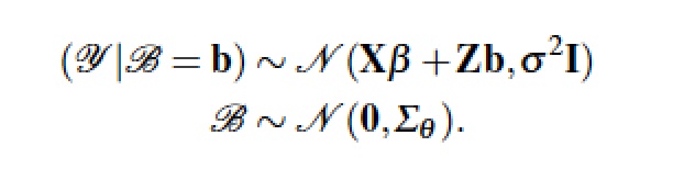
Laird and Ware (1982) (you can find the article here, but let me know if this link is broken) develop another popular form of the model in the equations above. In Stage 2, as they call the second level, the b matrix of unknown individual effects is distributed normally with covariance matrix D. The population parameters, the alpha matrix, are treated as fixed effects. In Stage 1, each individual unit i follows the second equation above: e is distributed N(0,R) where R is the covariance matrix. At this stage, the alpha and the beta matrices are considered fixed.
In the marginal distribution, (y | b), the y are also independent normals with covariance matrix R + Z D Z' where R, under conditions of conditional independence, can be simplified to an identity matrix with a single standard error, sigma.
The Laird and Ware (1982) article is worth detailed study. They present not only the ML model but also the Bayesian approach that leads to the restricted maximum likelihood (REML) estimator. And, they explain clearly how the EM (expectation-maximization) algorithm can be used to solve the model. The EM algorithm treats the individual characteristics of random effects models as missing data where the expected value replaces each missing data element after which the effects are re-estimated until the likelihood is maximized. I will talk about the EM algorithm in a future post because it is the best approach to deal generally with missing data.
 Finally, we get to Doug Bates' notation, which should be clearer now that we have presented the Laird and Ware model. What is important to note is that Doug assumes conditional independence.
Although I love matrix algebra, for HLMs I prefer to write out models explicitly in non-matrix terms as was done in the first set of equations above. In the lme4 package, my students have found the notation for specifying the random components of the model in the Z matrix to be somewhat confusing. Returning to the single-equation HLM form of their models has help to clear up the confusion.
The lme4 package has been developed by Doug Bates at the University of Wisconsin and is considered state-of-the-art for ML estimation of mixed models, that is, models with both fixed and random effects, such as hierarchical models. Package documentation is available here, draft chapters of a book on lme4 are available here and an excellent presentation on lme4 given at the UseR!2008 Conference is available here.
In Chapter 1 of the lme4() book, Doug Bates is careful to clear up the terminological problems that have plagued the statistics literature:
- Mixed-Effects Models describe a relationship between a response (dependent) variable and the covariates (independent variables). However, a mixed-effects model contains both fixed- and random-effects as independent variables. Furthermore, one of the covariates must be a categorical variable representing experimental or observational units (the units of analysis).
- Fixed-effect Parameters are parameters associated with a covariate that is fixed and reproducible, meaning under experimental control.
- Random Effects are levels of a covariate that are a random sample from all possible levels of the covariate that might have been included in the model.

To me, the confusion is cleared up by returning to the model and considering the terminology an attribute of the model rather than the data. In the model above, lambda 00 is the fixed effect and mu 0j is the random effect which is simply the error term on the first equation. Since both mu 0j and epsilon ij are error terms, they are not parameters in the model. On the other hand, sigma u0 and sigma e are parameters. Still confused?
What I will argue repeatedly in remaining posts is that the way you determine what is or is not a parameter is through Monte Carlo simulation. For a given model, terms that must be fixed before you can run the simulation are parameters. Other terms in the model are random variables, that is, simulation variables that we will have to generate from some density function. What I insist to my students is that you cannot use input data to run the Monte Carlo simulation. In order for the simulation to work without input data, you must be clear about (and often surprised by) the actual random variables in your model.
Before I present the ML model in the notation Doug Bates is using, let's return to the expanded Dyestuff hierarchical model introduced earlier.


In the marginal distribution, (y | b), the y are also independent normals with covariance matrix R + Z D Z' where R, under conditions of conditional independence, can be simplified to an identity matrix with a single standard error, sigma.
The Laird and Ware (1982) article is worth detailed study. They present not only the ML model but also the Bayesian approach that leads to the restricted maximum likelihood (REML) estimator. And, they explain clearly how the EM (expectation-maximization) algorithm can be used to solve the model. The EM algorithm treats the individual characteristics of random effects models as missing data where the expected value replaces each missing data element after which the effects are re-estimated until the likelihood is maximized. I will talk about the EM algorithm in a future post because it is the best approach to deal generally with missing data.
Although I love matrix algebra, for HLMs I prefer to write out models explicitly in non-matrix terms as was done in the first set of equations above. In the lme4 package, my students have found the notation for specifying the random components of the model in the Z matrix to be somewhat confusing. Returning to the single-equation HLM form of their models has help to clear up the confusion.
> fm1 <- lmer(Yield ~ 1 + (1|Batch),Dyestuff)
> summary(fm1)
Linear mixed model fit by REML
Formula: Yield ~ 1 + (1 | Batch)
Data: Dyestuff
AIC BIC logLik deviance REMLdev
325.7 329.9 -159.8 327.4 319.7
Random effects:
Groups Name Variance Std.Dev.
Batch (Intercept) 1764.0 42.001
Residual 2451.3 49.510
Number of obs: 30, groups: Batch, 6
Fixed effects:
Estimate Std. Error t value
(Intercept) 1527.50 19.38 78.81
The Dyestuff model is specified in the lme4() procedure with the equation Yield ~ 1 + (1|Batch). The random effects in the parentheses are read "the effect of Batch given the grand mean". It may seem strange to find the grand mean (represented by the 1) specified twice in a model. Going back to the single equation HLM form, notice that there are two constants, lambda 00 and the first element of the beta 0 j matrix, thus the two grand means.
Moving beyond the notation to the estimated values, we have two standard errors (42.001, and 49.510) and one fixed effect parameters, 1527.50 with standard error 19.38. The "Random effects: Residual" is the same residual standard deviation, 49.510, as from the OLS ANOVA. That's a little disconcerting because, they way the initial model was written, it would seem that the residual standard deviation should be smaller when we have taken the random error components out of the OLS estimate.
> coef(m1)[1] + mean(coef(m1)[2:6])
(Intercept)
1532
The fixed effect mean is very similar to the average of the OLS coefficients. So, all this heavy machinery was developed to generate the one number, 42.001. Here's my question: "Is this the right number?" I will argue in the next post that the only way to answer this question is through Monte Carlo simulation.
NOTE: Another way to think about random and fixed effects is to think about the problem of prediction. If we want to predict the Yield we might get from a future batch of dyestuff from some manufacturer, all we have to work with are the fixed part of the models. The random components are unique to the sample and will not be reproduced in future samples. We can use the standard deviations and the assumed density functions (usually normal) to compute confidence intervals, but the predicted mean values can only be a function of the fixed effects.
NOTE: Another way to think about random and fixed effects is to think about the problem of prediction. If we want to predict the Yield we might get from a future batch of dyestuff from some manufacturer, all we have to work with are the fixed part of the models. The random components are unique to the sample and will not be reproduced in future samples. We can use the standard deviations and the assumed density functions (usually normal) to compute confidence intervals, but the predicted mean values can only be a function of the fixed effects.
Monday, September 24, 2012
The Dyestuff Model
In a prior post (here), I introduced the Dyestuff data set. At first, one might be tempted to run an analysis of variance (ANOVA) on this data since the stated intention is to analyze variation from batch to batch. The ANOVA model is equivalent to the standard regression model.

Here, all the terms represent matrices: Y is an (n x 1) matrix of dependent variables, Yield in this case. X is an (n x m) design matrix (to be explained in the NOTE below) coding the Batch. The beta matrix is a (m x 1) matrix of unknown coefficients. And, the e matrix is an (n x 1) matrix of unknown errors (departures from perfect fit) distributed normally with mean zero and a single variance, sigma. If your matrix algebra is weak, R provides a great environment for learning linear algebra (see for example here).
The regression model is completely equivalent to ANOVA. You can convince yourself of this by running the two analyses in R.
In R, the anova(m1) command produces the same results as summary(m1), only the results are presented as the standard ANOVA table.
The naive regression result finds that the means of Batches C and E are significantly different from the other batches. What the result says for the initial question is that most batches are +/- 31.31 units from the average yield of 1505. However, some batches can be significantly outside this range. But, is this an analysis of means or analysis of variances? The history and development of terminology (analysis-of-variance, analysis of means, random error terms, random components, random effects, etc.) makes interesting reading that I will explore in a future post. To maintain sanity, it's important to keep focused on the model rather than the terminology.
If we write out another model that might have generated this data, it becomes easier to clarify terminology and understand why ANOVA (analysis of means) might not be the right approach to analyze the variation from batch to batch.


The regression model is completely equivalent to ANOVA. You can convince yourself of this by running the two analyses in R.
> m1 <- lm(Yield ~ Batch,Dyestuff,x=TRUE)
> summary(m1)
Call:
lm(formula = Yield ~ Batch, data = Dyestuff, x = TRUE)
Residuals:
Min 1Q Median 3Q Max
-85.00 -33.00 3.00 31.75 97.00
Coefficients:
Estimate Std. Error t value Pr(>|t|)
(Intercept) 1505.00 22.14 67.972 < 2e-16 ***
BatchB 23.00 31.31 0.735 0.46975
BatchC 59.00 31.31 1.884 0.07171 .
BatchD -7.00 31.31 -0.224 0.82500
BatchE 95.00 31.31 3.034 0.00572 **
BatchF -35.00 31.31 -1.118 0.27474
---
Signif. codes: 0 ‘***’ 0.001 ‘**’ 0.01 ‘*’ 0.05 ‘.’ 0.1 ‘ ’ 1
Residual standard error: 49.51 on 24 degrees of freedom
Multiple R-squared: 0.4893, Adjusted R-squared: 0.3829
F-statistic: 4.598 on 5 and 24 DF, p-value: 0.004398
> anova(m1)
Analysis of Variance Table
Response: Yield
Df Sum Sq Mean Sq F value Pr(>F)
Batch 5 56358 11271.5 4.5983 0.004398 **
Residuals 24 58830 2451.2
---
Signif. codes: 0 ‘***’ 0.001 ‘**’ 0.01 ‘*’ 0.05 ‘.’ 0.1 ‘ ’ 1
In R, the anova(m1) command produces the same results as summary(m1), only the results are presented as the standard ANOVA table.
The naive regression result finds that the means of Batches C and E are significantly different from the other batches. What the result says for the initial question is that most batches are +/- 31.31 units from the average yield of 1505. However, some batches can be significantly outside this range. But, is this an analysis of means or analysis of variances? The history and development of terminology (analysis-of-variance, analysis of means, random error terms, random components, random effects, etc.) makes interesting reading that I will explore in a future post. To maintain sanity, it's important to keep focused on the model rather than the terminology.
If we write out another model that might have generated this data, it becomes easier to clarify terminology and understand why ANOVA (analysis of means) might not be the right approach to analyze the variation from batch to batch.

Since we have no control over the sampling of batches, we expect that the Yield coefficient will have a random source of variation in addition to the true population yield (see the first equation above). Under normal experimental conditions we might try to randomize away this source of variation by sampling batches for a wide range of suppliers. But, since we are actually not using random assignment, we have a unique source of variation associated with the yield of each batch. As can be seen from the first equation above, this is where the term random coefficients comes from. Where we have random sampling, the effect of Batch on Yield would be a fixed effect, that is, fixed under sampling. In this model, the fixed effect is lambda_00 rather than the usual beta.
The equation that determines Yield (the second and third equations above) thus has a random coefficient. If we substitute Equation 1 into Equation 2, we get Equation 4. Notice that we now have a larger error term, one error associated with Batch and another associated with the model. The purpose of hierarchical modeling is to account for the source of error associated with how the Batches are generated. The "analysis of variance" here involves the two sigma parameters, sigma_u0 (the standard error of the yield coefficient) and sigma_e (the standard error of the regression).
What you might be asking yourself right now is "If this is a HLM, where's the hierarchy?" Let's assume that we were receiving batches from more than one manufacturer. Then, we would have batches nested within suppliers, but still no random sampling. To account for the effect of supplier, we need another second-level variable (second level in the hierarchy), Z, that is an indicator variable identifying the manufacturer.

The organizational chart above makes the hierarchy explicit. If we take the Z out of the model, however, we are still left with a random coefficients model. Since most human activity is embedded within some social hierarchy, it is hard to find a unit of analysis that is not hierarchical: (1) students within class rooms, classrooms within schools, schools within school systems, etc., (2) countries nested within regions, (3) etc. When these implicit hierarchies are not modeled, a researcher can only hope that the second-level random effects are small.
Returning to terminology for a moment, if we were just interested in the analysis of means, then standard ANOVA models (sometimes called Type I ANOVA) gives us a fairly good analysis of differences in Yield. We might have more error associated with the non-random Batches in the error term, but we still have significant results (some Batches have significantly different means in spite of the unanalyzed sources of Batch variance). However, if we are interested in true analysis of variance (sometimes called Type II ANOVA) and if we expect that there is some unique source of variation associated with Batches that we want to analyze, we need a technique that will produce estimates of both sigma_u0 (the standard error of the yield coefficient) and sigma_e (the standard error of the regression).
There are multiple techniques that will perform a Type II ANOVA or random coefficients analysis. In the next post I'll discuss the most popular approach, Maximum Likelihood Estimation (MLE).
NOTE: The equivalence of ANOVA and regression becomes a little clearer by looking at the design matrix for the Dyestuff model. Most students are familiar with the standard regression model where the independent variable, X, is an (n x 1) matrix containing values for a continuous variable. This is how the difference between ANOVA and regression is typically explained in introductory text books. However, if the X matrix contains dummy [0,1] variables coding each Batch, the regression model is equivalent to ANOVA. Here is the design matrix, as the ANOVA X matrix is often called, for the Dyestuff model:
> m1$x
(Intercept) BatchB BatchC BatchD BatchE BatchF
1 1 0 0 0 0 0
2 1 0 0 0 0 0
3 1 0 0 0 0 0
4 1 0 0 0 0 0
5 1 0 0 0 0 0
6 1 1 0 0 0 0
7 1 1 0 0 0 0
8 1 1 0 0 0 0
9 1 1 0 0 0 0
10 1 1 0 0 0 0
11 1 0 1 0 0 0
12 1 0 1 0 0 0
13 1 0 1 0 0 0
14 1 0 1 0 0 0
15 1 0 1 0 0 0
16 1 0 0 1 0 0
17 1 0 0 1 0 0
18 1 0 0 1 0 0
19 1 0 0 1 0 0
20 1 0 0 1 0 0
21 1 0 0 0 1 0
22 1 0 0 0 1 0
23 1 0 0 0 1 0
24 1 0 0 0 1 0
25 1 0 0 0 1 0
26 1 0 0 0 0 1
27 1 0 0 0 0 1
28 1 0 0 0 0 1
29 1 0 0 0 0 1
30 1 0 0 0 0 1
attr(,"assign")
[1] 0 1 1 1 1 1
attr(,"contrasts")
attr(,"contrasts")$Batch
[1] "contr.treatment"
Notice that there is no BatchA, since it plays the role of the reference class to which other batches are compared. That is, the coefficients attached to BatchB through BatchF are expressed as deviations from the grand mean (this construction is necessary because there are only 6 parameters and 6 degrees of freedom, so one class has to become the grand mean).
Saturday, September 22, 2012
A Simple HLM: The Dyestuff Example
Hierarchical Linear Models (HLMs) have their own terminology that challenges a lot of what is taught as basic statistics. We have random effects, random coefficients, and mixed-models added on to what we already know about random error terms and fixed effects. It will help to start with a simple data set that so we can introduce new terms one at a time.
The lme package in the R programming language has a simple data set that provides a good starting point. If you have R running on your machine and the lme package installed, typing help(Dyestuff) produces the following description of the data set:
The
Dyestuff data frame provides the yield of dyestuff (Naphthalene Black 12B) from 5 different preparations from each of 6 different batchs of an intermediate product (H-acid).
The
Dyestuff data are described in Davies and Goldsmith (1972) as coming from “an investigation to find out how much the variation from batch to batch in the quality of an intermediate product (H-acid) contributes to the variation in the yield of the dyestuff (Naphthalene Black 12B) made from it. In the experiment six samples of the intermediate, representing different batches of works manufacture, were obtained, and five preparations of the dyestuff were made in the laboratory from each sample. The equivalent yield of each preparation as grams of standard colour was determined by dye-trial.”
Notice that the batches are not randomly chosen out of some universe of manufactured batches. They are whatever we were able to "obtain". Just to make things concrete, here are the first few lines of the file printed by the R head() command (the > before the head command is the R prompt):
At first, one might be tempted to run an analysis of variance (ANOVA) on this data since the stated intention is to analyze variation from batch to batch. However, there are issues presented by this simple data set that help us understand the added complexity and potential benefits of hierarchical modeling.
In general, the standard approach is to move directly from a data set to some kind of estimator. In the next few posts, I will argue that the standard approach misses a number of important opportunities.
> head(Dyestuff)
Batch Yield
1 A 1545
2 A 1440
3 A 1440
4 A 1520
5 A 1580
6 B 1540
At first, one might be tempted to run an analysis of variance (ANOVA) on this data since the stated intention is to analyze variation from batch to batch. However, there are issues presented by this simple data set that help us understand the added complexity and potential benefits of hierarchical modeling.
In general, the standard approach is to move directly from a data set to some kind of estimator. In the next few posts, I will argue that the standard approach misses a number of important opportunities.
Sunday, September 16, 2012
The 'hlmmc' package
From July 1 through August 15, I taught Sociology S534 Advanced Sociological Analysis: Hierarchical Linear Models at the University of Tennessee in Knoxville. A syllabus for the course is available here. Over the next few months I will serialize the lectures and a user guide for the software package ('hlmmc') used in the course. 'hlmmc' is a software package written in the R programming language for studying Hierarchical Linear Models (HLMs) using Monte Carlo simulation. A manual for the software package is available here. It explains how to download the software and how each function in the package can be used (also, see NOTE below).
The approach I used in the course was to write out the equations for each linear model as a function in the R programming language. The functions were designed so that data for the study could be simulated for each observation in the sample. This is a useful exercise because it forces you to confront a number of difficult issues. What statistical distributions will be used to not only simulate the distributions of the error terms but also the distributions of the independent variables? Typically, a normal distribution is chosen for the error terms and the distributions of the independent variables are ignored in planning a study. Monte Carlo Simulation forces the researcher to confront these issues in addition to explicitly stating the functional form of the model, the actual parameters in the model and a likely range for the parameter values that might be encountered in practice.
In the next posting I'll start with a very simple hierarchical data set and develop an R function for simulating data from a model that could be used to generate similar data. The Monte Carlo function frees us from the sample data and lets us explore more general issues raised by the model. The pitch to my students was that the Monte Carlo approach would provide a deeper understanding of the issues raised by hierarchical models.
The basic feedback from students was that, in the short time available for the class, they were able to get a deeper understanding of HLMs than if the class had be structured as a conventional statistics class (math lectures and exercises?). One student comment in the course evaluations that s/he "...wished all stat classes were taught this way." For better or worse, my classes always have been.
If you are interested in the topic and want to follow the serialization in future postings, I will try to follow my lectures, which were live programming demonstrations, as closely as possible keeping in mind some of the questions and problems my students had when confronting the material.
NOTE: Assuming you have R installed on your machine and you have downloaded the files LibraryLoad.R and HLMprocedures.R to some folder on you local machine, you can load the libraries and procedures using the following commands in R:
where > is the R prompt and W is the absolute path to the working directory where you downloaded the files LibraryLoad.R and HLMprocedures.R. The Macintosh and Windows version of R have 'Source' selection in the File menu that will also allow you to navigate your directory to the folder where these two files have been downloaded. When you source the LibraryLoad.R file, error messages will be produced if you have not installed the supporting libraries listed in the manual (here).
The approach I used in the course was to write out the equations for each linear model as a function in the R programming language. The functions were designed so that data for the study could be simulated for each observation in the sample. This is a useful exercise because it forces you to confront a number of difficult issues. What statistical distributions will be used to not only simulate the distributions of the error terms but also the distributions of the independent variables? Typically, a normal distribution is chosen for the error terms and the distributions of the independent variables are ignored in planning a study. Monte Carlo Simulation forces the researcher to confront these issues in addition to explicitly stating the functional form of the model, the actual parameters in the model and a likely range for the parameter values that might be encountered in practice.
In the next posting I'll start with a very simple hierarchical data set and develop an R function for simulating data from a model that could be used to generate similar data. The Monte Carlo function frees us from the sample data and lets us explore more general issues raised by the model. The pitch to my students was that the Monte Carlo approach would provide a deeper understanding of the issues raised by hierarchical models.
The basic feedback from students was that, in the short time available for the class, they were able to get a deeper understanding of HLMs than if the class had be structured as a conventional statistics class (math lectures and exercises?). One student comment in the course evaluations that s/he "...wished all stat classes were taught this way." For better or worse, my classes always have been.
If you are interested in the topic and want to follow the serialization in future postings, I will try to follow my lectures, which were live programming demonstrations, as closely as possible keeping in mind some of the questions and problems my students had when confronting the material.
NOTE: Assuming you have R installed on your machine and you have downloaded the files LibraryLoad.R and HLMprocedures.R to some folder on you local machine, you can load the libraries and procedures using the following commands in R:
> setwd(W)
> source(file="LibraryLoad.R")
> source(file="HLMprocedures.R")
Saturday, March 10, 2012
Six Useful Classes of Linear Models
 Statistics (or Sadistics as my students like to call it) is a difficult subject to teach with many seemingly unrelated and obscure concepts, many of which are listed under "Background Links" in the right-hand column. Compare Statistics to Calculus, another difficult topic for students. In the Calculus there are only three concepts: a differential, an integral and a limit. Statisticians could only dream of such simplicity and elegance (have you finished counting all the concepts listed on the right)?
One way that has helped me bring some order to this chaos is to concentrate on the classes of models typically used by statisticians. The six major classes are displayed above in matrix notation (if you need a review on matrix algebra, try the one developed by George Bebis here). Clearly understanding each of the common linear models will also help classify Hierarchical Linear Models.
Equation (1) states simply that some matrix of dependent variables, Y, is the result of some multivariate distribution, E. The letter E is chosen since this distribution will eventually become an error distribution. The subscript, i, denotes that there can be multiple models for different populations--a really important distinction.
 Before leaving model (1) it is important to emphasize that we believe our dependent variables have some distribution. Consider the well-known distribution of Intelligence (IQ) displayed above (the "career potential" line in the graphic is a little hard to take; I know many police officers with higher intelligence than lawyers, but at least the graphic didn't use the "moron," "imbecile," and "idiot" classifications). It just so happens that the normal distribution that describes IQ is the same distribution that describes E in many cases. The point is that most dependent variables have a unimodal distribution that looks roughly bell-shaped. And, there are some interesting ways to determine a reasonable distribution for your dependent variable that I will cover in future posts.
Equation (2) is the classical linear model where X is a matrix of fixed-effect, independent variables and B is a matrix of unknown coefficients that must be estimated. There are many ways to estimate B, adding further complexities to statistics, but least squares is the standard approach (I'll cover all the different approaches in future posts). Notice also that once B is estimated, E = Y - XB by simple subtraction. The important point to emphasize here, a point that is often ignored in practice, is that X is fixed either by the researcher or is fixed under sampling. For example, if we think that IQ might affect college grade point (GPA) as in the model introduce here, then we have to sample equal numbers of observations across the entire range of IQ, from below 70 to above 130. Of course, that doesn't make sense since people with low IQ do not usually get into college. The result of practical sampling restrictions, however, might change the shape of the IQ distribution, creating another set of problems. Another way that the independent variables can be fixed is through assignment. When patients are assigned to experimental and control groups in clinical trials, for example, each group is given a [0,1] dummy variable classification (one if you are in the group, zero if not). Basically, the columns of X must each contain continuous variables such as IQ or dummy variables for group assignments.
Equations (3-6) start lifting the restriction on fixed independent variables. In Equation (3), the random (non-fixed) variables are contained in the matrix Z with it's own set of coefficients, A, that have to be estimated. Along with the coefficients, random variables have variances that also must be estimated, thus model (3) is called the random effects model. Typically, hierarchical linear models are lumped in with random effects models but in future posts and at the end of this post, I will argue that the two types of models should be thought of separately.
Equation (4) is the two-stage least squares model often used for simultaneous equation estimation in economics. Here, one of the dependent variables, y, is singled out as of primary interest even though there are other endogenous variables, Y, that are simultaneously related to y. Model (4) describes structural equation models (SEMs, introduced in a previous post here) as typically used in economics. The variables in X are considered exogenous variables or predetermined variables meaning that any predictions from model (4) are generally restricted to the available values of X. Again, there are a number of specialized estimation techniques for the two-stage least squares model.
Equation (5) is the path analytic model used in both Sociology and Economics. In the path analytic SEM, all the Y variables are considered endogenous. Both model (4) and model (5) bring up the problem of identification which I will cover in a future post. Again, there are separate techniques for the estimation of parameters in model (5). There are also a whole range of controversies surrounding SEMs and causality that I will also discuss in future posts. For the time being, it is important to point out that model (5) starts to look at the unit of analysis as a system that can be described with linear equations.
Finally, Equation (6) describes the basic time series model as an n-th order difference equation. The Y matrix, in this case, has a time ordering (t and t-1) where the Y's are considered output variables and the X's are considered input variables. Time series models introduce a specific type of causality called Granger causality, for the economist Clive Granger. In model (6) the Y(t-1) variables are considered fixed since values of variables in the past have already been determined. However, the errors in E can be correlated over time introducing the concept of autocorrelation. Also, since time series variables tend to move together over time (think of population growth and the growth of Gross National Product), time series causality can be confounded by cointegration, a problem that was also studied extensively by Clive Granger.
Models (1-6) don't exhaust all the possible models used in Statistics, but they do help classify the vast majority of problems currently being studied and do help us fix ideas and suggest topics for future posts. In the next post, my intention is to start with model (1) and describe the different types of distributions one typically finds in E and introduce some interesting approaches to determining the probable distribution of your data. These approaches differ from the typical null-hypothesis testing (NHT) approach (here) where you are required to test whether your data are normally distribution (Step 3, Testing Assumptions) before proceeding with conventional statistical tests (a topic I will also cover in a future post).
Finally, returning to the problem of hierarchical linear models (HLMs), the subscript i was introduced in models (1-6) because there is a hierarchical form of each model, not just model (3). The essential idea in HLMs (see my earlier post here) is that the unit of analysis is a hierarchical system with separate subpopulations (e.g., students, classrooms, hospitals, patients, countries, regions, etc.). Aspects of the subpopulations could be described by any of the models above. The area of multi-model inference (MMI) provides a more flexible approach to HLMs and solves the problems introduced by Simpson's paradox (described in an earlier post here).
MMI can be used successfully to determine an appropriate distribution for your data and help avoid the dead-end of NHT assumption testing. I'll cover the MMI approach to Equation (1) above in the next post. The important take away for this post is that determining the class or classes of models that are appropriate to your research question will help determine the appropriate type of analysis and types of assumptions that have to be made to complete the analysis.
Friday, February 17, 2012
Peeking, Tweaking and Cross-Validation
The classical Null Hypothesis Testing (NHT) paradigm (see my prior posts on NHT here) is focused almost exclusively on the critical experiment. The critical experiment, for example the gold-standard clinical trial, is set up to insure that a hypothesis is given a definitive test. Does administration of a drug actually produce a significant reduction in the target disease. Competing explanations are controlled through random sampling and random assignment. Subjects are chosen randomly from some population and are assigned randomly to treatment and control. There may actually be multiple control groups, some receiving placebos, some receiving competitor drugs and others receiving nothing. For this purpose, classical NHT is well suited, if not not very cost effective.
In the everyday world of science, however, classical NHT is easy to teach but hard to implement. Research, by its very definition, is mostly exploratory. Any interesting scientific question starts as a somewhat poorly formed idea. Concepts are a little unclear. Measurement of the concepts are open to question. Causal processes may be obscure and even unobservable. There needs to be a period of exploration, development and more casual testing. A lot of this period will involve exploratory data analysis.
Unfortunately, NHT doesn't really allow data exploration. Significance tests and associated probability levels are based on the assumption that you have not peeked at your data. The probability levels also assume that you have not estimated your model once, found it inadequate and gone on to tweak the model until it fits your sample data. In other words, NHT assumes that you are not involved in post-hoc analysis. Is there a solution to this dilemma?
In preparation for a research project I'm currently working on, I started re-reading the literature on Path Analysis. I haven't worked in this area since the 1980's, so I started back there and began reading forward. I ran into a 1983 article by Norman Cliff titled Some Cautions Concerning the Application of Causal Modeling Methods. In the article, a number of interesting general points are made that make the article seem quite current.
To the problem of peeking and tweaking, a strong recommendation is made to use cross-validation. In cross-validation, a large sample is drawn, larger than is needed for adequate statistical power. Part of the sample is then sub-sampled and used for exploratory model development. The remaining part of the sample is used to test the tweaked model. Since one has not peeked at this data, there is the possibility of fairly testing the validity of the model, that is, cross validating the model.
The project I am currently working on involves studying Globalization in Latin America. Multi-country analysis provides another type of cross-validation. In this case, the principal investigator has extensive expertise on a few countries, the greatest expertise being in Mexico. Since a lot of his understanding of the research problem is based on experience in Mexico, one approach would be to use Mexico as the model development laboratory. Another approach would be to take some other country, say Argentina, and develop there using ones understanding of Mexico to guide model development. This approach could possibly produce a somewhat more general model.
In a future post, I will talk about how cross-validation worked in this specific context. I will also talk about the issue of statistical power analysis and sample size determination if a cross-validation is being attempted. There are also a number of other interesting points in the Cliff(1983) paper, particularly on causality, that would be worth discussion.
Subscribe to:
Posts (Atom)